Loading...

Ideas

Have an idea? Don't know where to start? We can help. We work with you to deeply understand your challenges, and identify the best path forward.

Algorithms

We turn your idea into carefully implemented algorithms and business logic that can be seemlessly integrated into your existing workflows.

Prototypes

The first step is the hardest. We create a working prototype to help you validate your idea, and test the market.

Stories

Even the best ideas need to be shared to have an impact. We target your audience and explain your product with the appropriate level of technical detail.

About Us

We apply mathematics and software engineering to solve technical problems and help companies understand the complex systems they rely on.

We provide expertise in mathematics and software development to automate time consuming manual processes and optimize the computational algorithms their work relies on.

We have applied these skills to support the United States Department of Defense, to automate a 6 hour manual data labelling task, and create visualizations of brain activity.

With experience ranging from fundamental research through software development we can easily integrate with any team in the organization and effectively communicate with stakeholders of all levels of technical knowledge.

Selected Projects

Identifying NFL player Positions

Automating a 6 hour process
Locally Adaptive Time Stepping

Improving the efficiency of large scale simulations
Modeling the Initiation of Type 1 Diabetes
Understanding Influence

Identifying trends in meeting records

Want to work with us?

We are always open to interesting projects.

Send us a message

Meet Our Team

Member Photo

Math and Computer Science

Richard Kublik

Principal Consultant

Richard has a particular skill in translating complex mathematical and analytical concepts into robust software prototypes. His speciality truly is in problem solving and execution.

Derek Doran

Tenet3, Director of R&D
Richard is always committed to the project's success and works diligently to solve problems and communicate the solution so that others on the team understand. Smart and a clear communicator, Richard is always fun to work with.

Rob Keefer

Pomiet

What’s the difference between a tight end and a receiver?

Turns out this is the hardest question in NFL football.

Football players lined up at the start of a play

Well, maybe not, but it was the trickiest question of a project I worked on.

I helped a football analytics company automate their data labelling process. For every play, in every game, all season long, the data labeling team paused the recording and identified the players on the field and what position they played. Sounds easy: check the team roster, scan the numbers on the jerseys, and done. Not quite. There are times when players are in a different position for a play, or you can’t see the jersey clearly. The annotation manual suggests identifying players using other features than their uniform, like the color of their shoelaces for example. Not so easy.

Life got better when the NFL started tracking the players. Now, each player’s location on the field is recorded multiple times per second. My project was to take the tracking data, and the guidebook and create an algorithm to label all the players, without looking at their shoelaces.

Once the quarterback was identified, most of the offensive positions were straightforward: the center directly in front, guards and tackles on either side. Wide receivers at the outer edges. For the defensive positions, the guide book described very clear regions relative to the offensive players and depth from the line of scrimmage. Depths are hard to estimate on the TV, easy when you’ve got the exact positions of everyone.

Now, back to the tight end: not part of the offensive line, but not a wide receiver either. According to the guidebook, a tight end has one hand on the ground, a wide receiver has no hands on the ground. Easy enough when you can see the players. The tracking data doesn’t include hand positions though. Fortunately, we had access to a full year’s worth of labeled data. Some quick analysis helped identify a threshold distance. Players within this distance of the offensive linesmen were tight ends, outside wide receivers. Not a perfect solution, but the client identified a threshold they were happy with.

In the end, the algorithm did very well. It took many iterations, comparisons to the existing labels, and discussions with the client to identify some of the nuances that were tripping us up. I made a visualization tool that helped immensely, and we even found some instances where the existing labels were incorrect. By the time the next football season started, the client had a working solution that they trusted.

I had more fun on this project than I initially thought I would. I’m not really into sports, and (still) have never watched a football game. It was a bit of a running joke at the beginning, but the project really wasn’t about football. The project was about understanding the data, extracting the important information from it, and delivering a working solution. That I can do.

Don’t wait for me, I’ll catch up

Simulations of electrical activity in nerve cells rely on solving large systems of non-linear differential equations thousands of times for each second of simulated time. These simulations can help us better understand how parts of the brain work, but they are very time consuming and computationally expensive.

There are two main components to the computational cost: the size of the physical domain which corresponds to how many equations are in the system; and how many times we need to solve the equations. There is a parameter referred to as stepsize that controls the second of these: the smaller the stepsize, the more times we need to solve the system of equations. In general, a system that evolves quickly (has a high activity level) requires a small time step to accurately capture the changes.

In the most naive approach, the stepsize is constant for the entire simulation, and is determined based on the highest activity level expected at any time during the simulation. This is simple to implement, but leads to extra work if the system evolves slowly except during a short time within the simulation.

A more refined approach is to use an adaptive time step. At each update, the stepsize selected is based on the fastest evolution at that instant, anywhere in the physical domain. This can reduce the computational cost, and isn’t much more complicated to implement than the first method. In fact, like the first method, there are standard packages available in most computational libraries to do this.

Sometimes in neural simulations the system of interest is very large, but there are only a small number of regions with high activity at any time. Most of the system could be simulated with a large stepsize, but since there is always some region with high activity, the simulation needs to select a small stepsize. As a graduate student, I developed an algorithm for these cases.

I developed an algorithm for locally adaptive time stepping (LATS). Within this scheme, the spatial domain is split into subdomains, and each subdomain is updated with an adaptive time step most appropriate for the local level of activity. Each subdomain evolves at its own pace, and waits for its neighbors to catch up. The challenge is in maintaining accurate flow of information and stability of the solution.

Through the application of domain decomposition techniques, I was able to computationally connect the subdomains through boundary conditions obtained through a conservation of flux. To address the stability concerns, I replaced the time stepping scheme that had been used for neuroscience simulations since the 1960s with a method that provides better stability and proved better suited to the LATS algorithm.

Evaluating the LATS algorithm is not as simple as stating an X% reduction in computational time. The underlying numerical scheme is comparable to the standard approach, but the major benefit of the LATS method is that the computational cost scales with the level of activity in the system, rather than the physical size of the domain. Thus in situations where there is sparse activity in a large computational domain, the LATS method provides a significant reduction in computational cost by focusing computational resources where they are most needed. The LATS method was developed within the context of computational neuroscience, but is applicable to any system with sparse activity.

In the animation below, an electrical impulse is initiated in a cell, and propagates through two cells. The colors represent the voltage, and the sections of the cell become transparent as the step size increases.

Electrical pulse travelling through two nerve cells.

A model for the early stages of type 1 diabetes

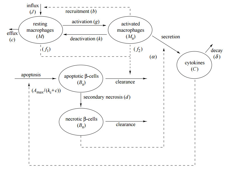
Type 1 diabetes occurs when the immune system attacks and destroys the insulin producing beta-cells in the pancreas. Our experimental collaborator had observed that macrophages (a part of the immune system that clears away dead cells from tissues) from mice susceptible to type 1 diabetes were less efficient than macrophages from healthy mice. It was also observed that not every mouse susceptible to the disease developed it. Based on these observations, we developed a model to answer two questions:

Can the difference in macrophage efficiency account for the differences observed between healthy and susceptible mice?
Can a naturally occurring wave of beta-cell death associated with normal development in all mice be a triggering event that leads to type 1 diabetes in susceptible mice?

schematic diagram of mathematical model

Within our modeling framework, the healthy state corresponds to a steady-state solution representing no inflammation, while the diseased state corresponds to a steady-state solution representing chronic inflammation. It is then assumed that during the chronic inflammation state the immune system will become primed to attack and kill the pancreatic beta-cells. Since not all susceptible mice develop type 1 diabetes, the healthy state should exist and be stable for both strains of mice being modeled. In addition, the steady state corresponding to chronic inflammation should exist and be stable for the susceptible mice. Through the use of dynamical systems approaches (especially phase-plane analysis) we determined that the initial model could not satisfy these requirements for biologically reasonable parameter values. The model was then expanded to include additional cell populations as well as the toxic effect of harmful cytokines released by the macrophages. This expanded model, shown below, demonstrated that differences in macrophage efficiency could explain the difference between healthy and susceptible mice.

To answer the second question, the wave of beta-cell death was incorporated into the model. The model demonstrated that for healthy mice the temporary inflammation quickly died down, and the model returned to the non-inflamed steady state. In the case of the susceptible mice, the wave of beta-cell death was sufficient to push the system to chronic inflammation, suggesting that the naturally occurring cell death could indeed be a triggering stimulus for the development of type 1 diabetes.